Electric Network Frequency Analysis 2.0
(Co-Author: Yannick Meyer)
Introduction
The grid frequency is usually used for the analysis of grid conditions in the European interconnected system. For example, we have recently analysed effects such as the grid split on 08 January 2021 or the RESA of the Krško nuclear power plant on 29 December 2020. The grid frequency can be understood as the heart line of the largest machine in the world. Just as the heartbeat can be measured in every cell of the human body, it can also be detected in every cell in the interconnected system, be it at the line, at a generator or a consumer. Because all devices, systems and machines connected to the grid only work because they (have to) run exactly at the same frequency as the grid. However, it is precisely this property that allows the grid frequency to be used as a measure of the location of events. Because just as the human pulse is not perfect, the grid frequency is not perfect either. Unique patterns emerge when you look at the frequency over time. And these patterns do not repeat, at least not in short successive intervals.
This uniqueness of the network frequency is used in the Electric Network Frequency Analysis (ENF Analysis) to classify events in time. For example, such a pattern is recorded with every audio or video recording if there is an active power consumer in the vicinity of the recording. This can be a switched‐on lamp, the PSU or other sound‐emitting consumers. However, due to the depth of the frequency and the low volume, we do not perceive this phenomenon with the human ear.
Microphones, on the other hand, can record the fundamental frequency or one of its harmonics around 100 or 200 Hz, depending on the microphone design. The mains hum recorded in this way can be used for the temporal classification of the recording to be evaluated, provided that an independent recording of the mains frequency is available with sufficiently high accuracy and temporal precision.
The Gridradar Monitoring System offers this possibility. This is because all measuring stations of the Gridradar system are synchronised in time through a Global Navigation Satellite System receiver (GNSS receiver). This means that the time stemp is identical across all measuring stations up to a few microseconds. Without corresponding GNSS tracking, e.g. using the NTP internet protocol, the frequency development in Europe cannot be clearly compared across different measuring stations. The time offset becomes clear in the following figure:
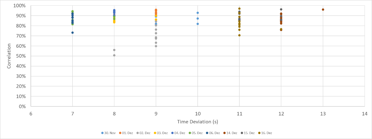
The figure shows a series of tests in which the grid hum isolated from recordings was compared with the frequency measured by Gridradar. For each recording, the NTP time measured was compared with the UTC time transmitted by GNSS. The figure shows a temporal offset of between seven and 13 seconds, with the offset varying between the days of the recordings. For example, the offset was lower on 6 December than on 14 December.
It also turned out that when readjusting the NTP time, a very high agreement with the mains frequency can be achieved. It should be noted that the readjustment was made to seconds and not milliseconds. A drift of the NTP time was also detected during the experiment. This drift in turn affects the correlation between the audio recording and the mains frequency.
ENF analyses of audio files in a field experiment
In the second half of 2020, different investigations were carried out to determine the recording period of test audio files. First, the mains frequency or a harmonic was isolated from an audio file. This is done by a so‐called Fourier transformation. The relevant frequency band is thus filtered out of the entire frequency spectrum of a recording. With the help of so‐called cross‐correlations between the isolated frequency and the mains frequency, it is then possible to check when a recording was made. To do this, the "frequency snippet" of the audio file is "pushed" over the mains frequency. At each point of comparison, the correlation coefficient of the frequency snippet of the recording with the mains frequency is formed. The following figure shows the results of a comparison over ten days at the last point in time of the comparison period.
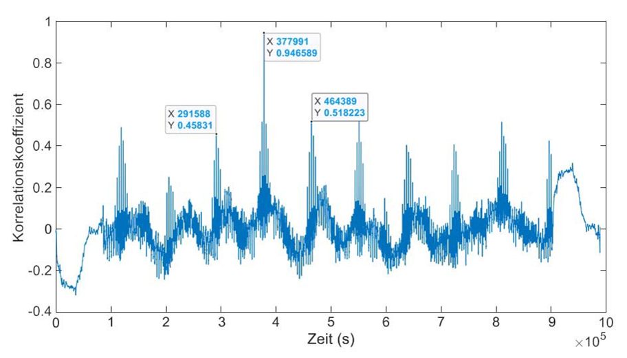
The following findings were thus obtained:
- Typical patterns emerge over the day regarding the correlation between the frequency of the audio file and the mains frequency. The correlation is always highest in the same period.
- The time window with the highest match each day is almost always identical to the actual recording time window.
- The highest correlation by far is with the actual recording time window.
Who is already using the ENF analysis?
ENF analysis is used in forensics, for example, to identify the period of time when a recording was made by police or investigating authorities. Therefore, forensic authorities use ENF analysis in the context of identifying the time window and continuity of a recording. Thus, it can be analyzed if a recording has been cut or compiled.
But ENF analyses are also used in journalistic research in order to be able to check the recording of leaked informant videos or audios for their authenticity, recording time and continuity.
For whom is the ENF analysis interesting beyond?
The ENF analysis is mainly used for the temporal identification of audio recordings when it comes to checking the authenticity of sound recordings. Especially in the context of so‐called deep fakes, audio or video recordings are "artificially" created. The ENF analysis is a proven and simple means of investigating the authenticity of recordings. For example, it could easily have been used to find out that Mrs. Pelosi was not drunk (https://www.youtube.com/watch?v=EfREntgxmDs). This is because this video was simply played slowed down to create a false impression. Here, a discrepancy between the mains hum of the recording and independent mains frequency recording would have been noticed.
However, the ENF technology can also be used in the opposite direction to define a unique time stamp. Therefore, audio or video files, for example, can be time‐signed specifically with the help of the frequency. This is relevant when a sequence of actions needs to be documented, such as in short‐term stock exchange trades.
Of course, this also opens up the possibility of using it in an insurance context, if the course of damage has to be classified in terms of time. Evidence presented to the insurer can also be checked for possible discontinuities, i.e. whether the evidence has been shortened or otherwise falsified by deliberate cuts.
What does Gridradar do?
Up to now, ENF technology has mainly been used as an ad‐hoc method. This requires extensive prerequisites, such as the prior delimitation of the time period of a recording, the procurement of the grid frequency and the precise investigation including the programming of the necessary analysis programme. Therefore, the method is only used to a very limited extent.
Gridradar offers an automated application of ENF technology, which can provide a good indication of the temporal location of an audio or video recording at short notice.
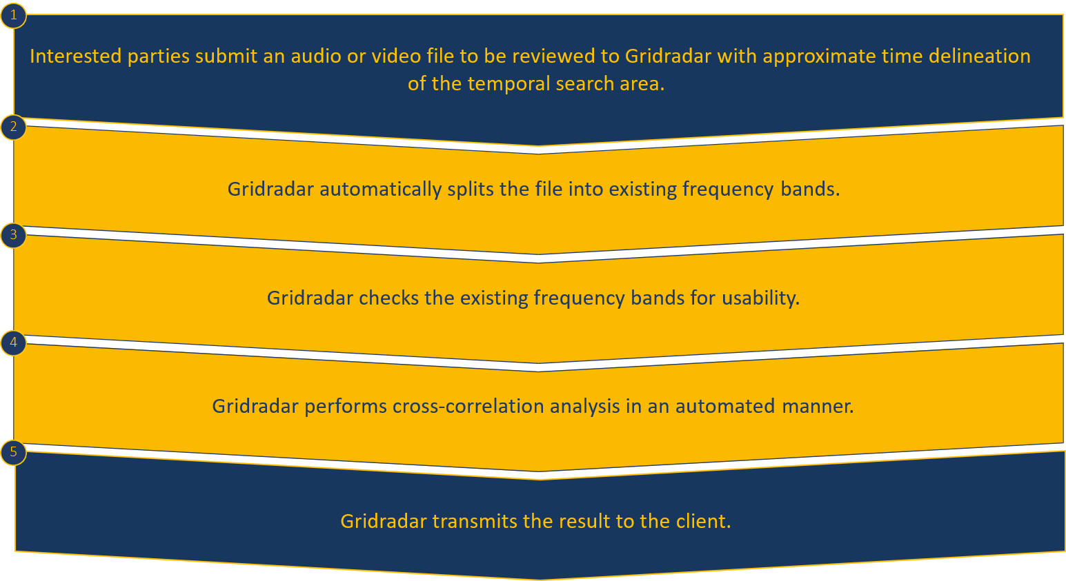
By standardizing and automating the process, results can be provided within a short period of time.
Gridradar thinks one step ahead
Certain regional patterns are recognizable in the grid frequency records. For example, the presence of large flywheel masses, such as a turbine set of a thermal power plant causes regional damping effects. These regional variations are only weakly recorded in the frequency, but influence the dispersion of the recorded frequency at a location. (Global Frequency Average – Regional Scatter?)
Gridradar's measurement system, which is distributed in the UCTE area, makes it possible to regionally classify these scatterings within a recording. Thus, by means of the ENF analysis, a recording can not only be classified in time and checked for continuity, but can also be located with a certain probability.