global frequency average - regional scatter

Initial considerations about frequency scatter

The frequency is considered to be approximately identical throughout Europe. Differences can only be found if a very high temporal resolution is selected in the display of the frequency. While in the seconds range the frequency still looks approximately identical, small differences appear in the tenths of a second range. This is true for the normal course of the day as well as for special events.

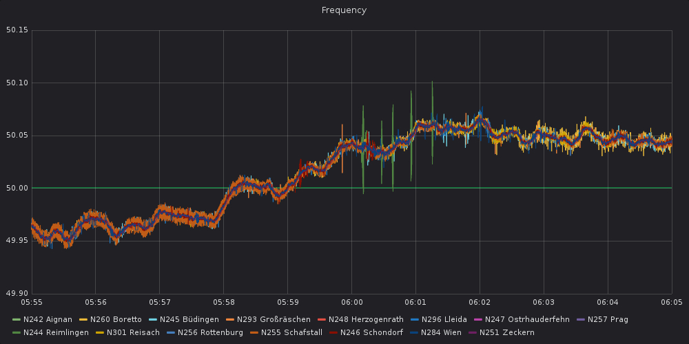
Above figure shows a typical frequency response, here on 01/16/2019, between 06:55 and 07:05. You can see the classic frequency increase in the morning hours towards the hourly break. Shown are the raw data of several measuring stations. All run approximately the same. Small jumps either indicate switching in the network or can be justified by very short-term disturbances that can occur due to the measurement in the distribution network. These deviations are normal.

However, a closer look reveals that the fluctuations of the individual lines vary. This becomes even more obvious when zooming into a shorter time window.

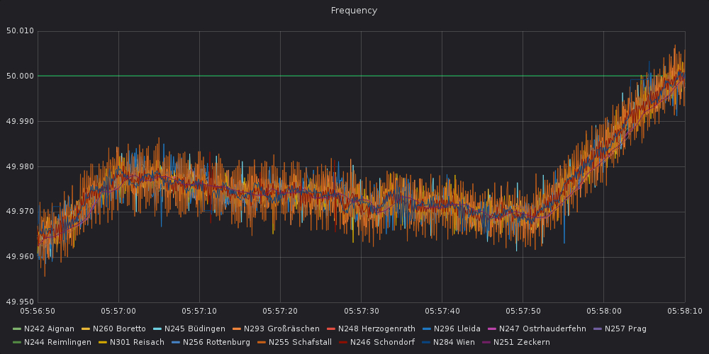
The figure shows the area between 06:57 and 06:58. While a red line in the middle hardly fluctuates, the blue and orange lines bounce around the red line more or less regularly in time and amplitude. Between the two extremes one sees other lines.

This observation raises the question of whether frequency fluctuations of individual measuring stations follow certain patterns, while the average frequency between measuring stations is identical. Such fluctuations indicate regional specifics. For example, in heavily industrialised regions, a stronger fluctuation could be expected due to short-term start-up and shut-down of large consumption plants, or one could possibly expect fluctuations due to the time of day or week of the producers connected to the grid. These considerations will be explored in the following.

measure of frequency scattering

As a measure of dispersion, we use the standard deviation of the frequency, sigma f, over a span of five seconds

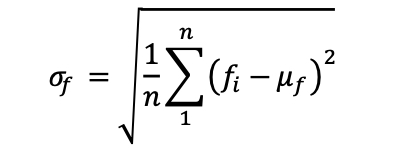
Sigma f is the root of the mean square deviation of the individual values from their arithmetic mean. Therefore it is always positive. The stronger the scatter, the larger sigma f.

We consider the half-year from November 2018 to April 2019. In order to be able to exclude statistical effects of frequency measurement, only measurement data from stations recording in the tenth of a second range are used for the analysis. These specifications mean that each analysis value is generated from measured values.

We have also tested alternative analysis methods, e.g. with a longer time window or other scattering measures. However, the central statements do not depend significantly on the method.

General observations

First, it must be clarified whether frequency fluctuations are random or whether there are systematic differences between measuring points. For this purpose, an overall view is taken in a first step.

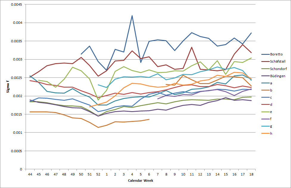
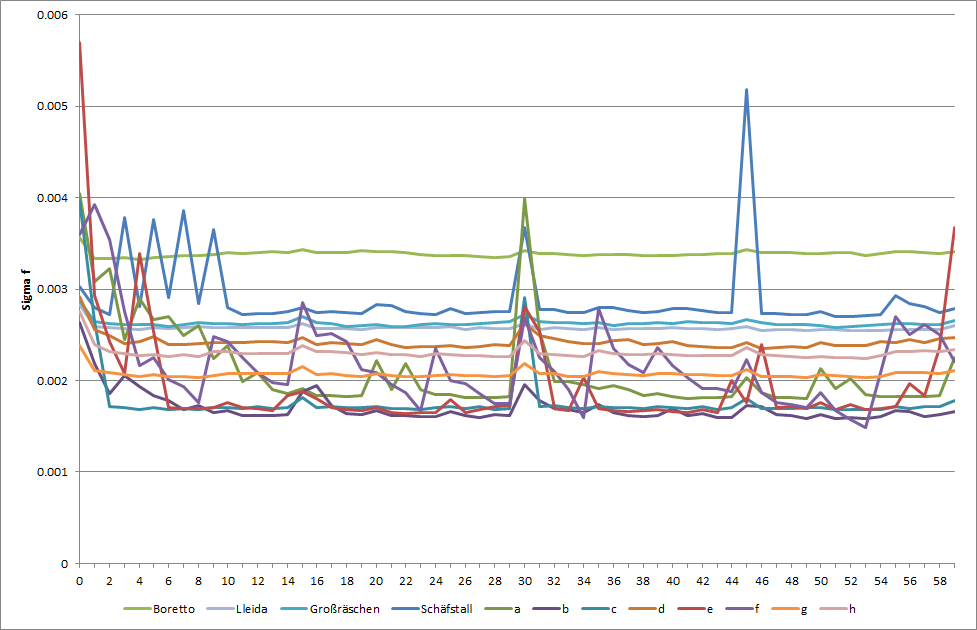
The figure shows the weekly average sigma f of the analysed measuring stations. At first glance, the observation made in the case study above is confirmed: Obviously, there are regions where there is a stronger fluctuation in frequency, such as around Boretto or Schäfstall, and those with comparatively little fluctuation, such as Schondorf and Büdingen. It also shows that the distribution of the variation over the measuring stations remains approximately the same over time. This means that the patterns are stable over time, with the scatter being greater at measuring stations with higher sigma f than at those with lower sigma f. On closer inspection, it can be seen that there is obviously less fluctuation in the Christmas week and that this then increases overall.

Transmission system operators explain these general fluctuation differences by the fact that frequency fluctuations in the centre of a network should be weaker on average than at the edges of the network. We also make this observation because, for example, the measuring station in Boretto, relatively far south, or the one in Lleida, relatively far west, record stronger frequency fluctuations in the European interconnected system. However, if we look at Schäfstall or Großräschen, both in Germany, at the centre of the interconnected grid, there seem to be additional local effects. Großräschen, for example, is located on the edge of the Lusatian lignite mining area.

Temporal pattern recognition

While the preceding analysis shows general differences in fluctuation, the following is concerned with effects in typical time intervals.

a) Weekdays

Weekdays typically differ in terms of energy consumption and thus energy production. On working days, more power is called up during the day. This power demand also starts earlier than on weekends or holidays. One can also recognise certain associated fluctuations in the frequency. For example, the morning ramp is usually accompanied by a frequency jump upwards to the hourly breaks, while in the evening hours one sees a frequency drop to the hourly breaks. (see German renewables have stabilising effect und long term analysis of renewables damping effect). These observations are more or less the same across Europe.

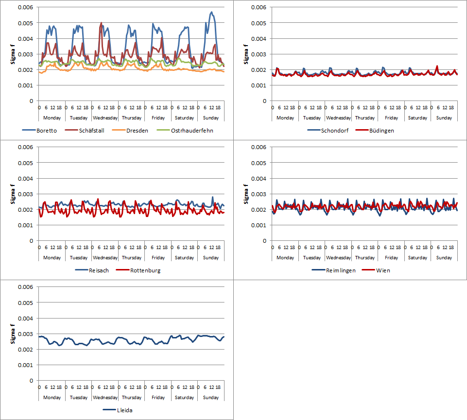
What surprised us, however, was that the frequency dispersion also follows certain patterns. These patterns differ between the measuring points. As an example, we have shown five patterns above.

The scattering patterns in the top left figure are very similar to the frequency patterns. During the day, the scattering is higher than during the night. In part, the two-hump pattern known from energy consumption can be recognised here. The difference between the points lies in the intensity of the pattern. Boretto and Schäfstall also show a very strong contrast between day and night hours.

The figure at the top right also shows the two-hump pattern. However, the amplitude in the morning hours is greater than that in the evening hours. In contrast to the first figure, the frequency dispersion over the day and over the night is similarly large. In addition, the comparison shows that at these measurement points the morning peaks occur somewhat earlier and the evening peaks somewhat later.

In the centre left figure we also see the two-hump structure with a slightly earlier second peak. The figure in the middle right shows a three-hump curve with much less frequency dispersion in the night hours.

Lleida differs completely from the other figures, as here there is generally a higher frequency dispersion in the off-peak hours (nights and weekends).

The differences in frequency scatter suggest that regional differences in consumption and generation could have an influence on the dispersion. The curve from Boretto suggests that as heterogeneous demand increases, so does the uncertainty in demand. The curve of Büdingen near Frankfurt, on the other hand, shows quite homogeneous demand with increased short-term uncertainty in the early morning hours when the data centres around Frankfurt are ramped up. The higher night-time uncertainty in Lleida can probably only be explained by the combination of lower night-time demand and wind availability in Spain. Due to the lower nightly demand, fewer conventional power plants are available. This makes it more difficult to compensate for fluctuations. Another assumption could be that the Spanish transmission system operator REE accepts more volatility during off-peak hours. However, this conjecture must be verified by further frequency recorders in Spain.

(At this point, we would like to point out that we are very interested in expanding the measurement system outside Germany and would appreciate your support. Please contact us if you are interested: info@gridradar.net.)

b) Course over the hour

From the frequency analysis it is known that strong frequency jumps](/en/blog/post/long-term-analysis-grid-frequency-proves-renewable-damping-effect-on-grid) happen at the [change of hour. In the course of the hour, stronger frequency changes, however, occur only rarely. Therefore, it is assumed that such frequency changes are mainly caused by the current market design with hourly products. (ENTSO-E will soon publish an analysis on market-related influences on grid stability). Frequency jumps, i.e. deviations in frequency, should also lead to a greater dispersion of frequency.

We have presented our analysis results in the following figure:

Even more than in the pure frequency analysis, the picture shows the typical exchange products with strong frequency dispersions at the hourly changes, but also at the half hours and, less pronounced, at the quarter hours. For example, hourly products dominate the markets in Spain and Italy, and half-hourly products in Italy. In Germany and - for historical reasons - in Austria, on the other hand, intraday trading with its quarter-hourly products already plays a greater role, which is why the spikes at these measuring stations are to be found at the quarter hours.

Strong regional differences can also be seen in the hourly view. The regionally different types of power plants seem to play a role here. The measuring station in Großräschen on the edge of the Lusatian mining area records only slight fluctuations over the hour and also at the hourly break. The operation of lignite-fired power plants can only be adjusted slowly. Therefore, they tend to operate continuously and dominate the regional impact on frequency due to their generation capacity. The measuring station in Schäfstall, on the other hand, records the operation of the river power plants on the Lech. These are much smaller in terms of output, but can also be used much more flexibly. The frequency dispersion especially at the hourly break shows that this flexibility is also actively used. But their flexibility is also in demand at the half hour and the third quarter hour.

c) hourly transition

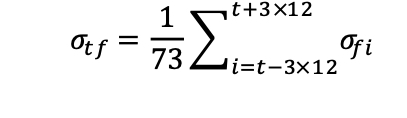As shown in previous studies, the hour break is of particular importance, whereby the frequency changes vary over the hours of the day. We have chosen the time window from three minutes before to three minutes after the hour break for the following consideration. This corresponds to the range in which the hour-related frequency change begins and ends. The following figure shows the average 5-second standard deviation in the interval three minutes before to three minutes after the hourly break for each hour.

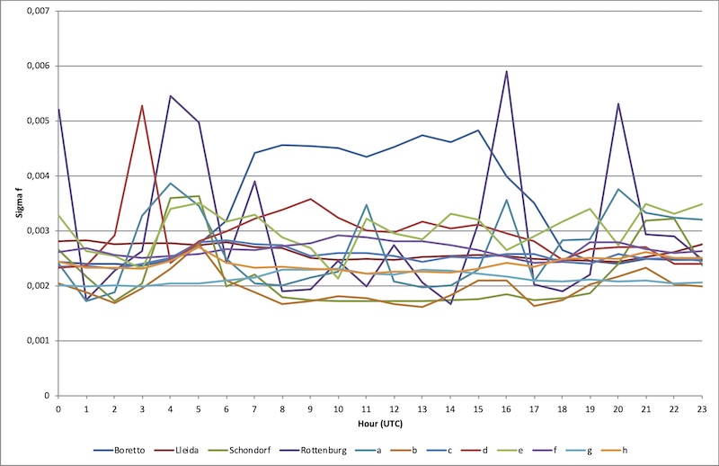
Here again, the picture is very heterogeneous with some measuring stations where the hourly fraction-related frequency dispersion remains more or less the same over the course of the day and others where the frequency dispersion varies over the course of the day.

As an example, we look at three measuring stations with special patterns:

• The recorder in Boretto records a higher frequency dispersion over the daytime hours than over the nighttime hours. From the comparison with the daily development over the week (see above), it becomes clear that the frequency dispersion in Boretto is less related to the hourly break than to the time of day.

• Schondorf shows two strong spikes in the times of highest energy demand in the morning and in the evening, while the frequency dispersion over the day and in the night hours is rather low. It can be assumed that this pattern is due to the proximity of the measuring station to Munich. The relatively early first deflection and the relatively late second deflection during the course of the day indicate that these are diurnal changes in power plant operation.

• We cannot explain the strong excursion of the measuring station in Lleida at 03:00. It is neither a statistical "outlier effect" nor the result of several individual events.

Conclusion

Frequency is an indicator of system stability in the European interconnected system. It follows an approximately similar course across regions. However, if we look at its dispersion, we see large differences between regions.

In the previous study, the half-year from the beginning of November 2018 to the end of April 2019 was taken as an example. It can be shown that the scattering identified is not random but systematic and differs from region to region. On the one hand, there are general differences in the strength of the scatter, which, however, remain more or less the same over time. Measuring stations with weaker frequency dispersion at the beginning of the observation period remain in the lower dispersion range over time. Those with stronger scattering at the beginning remain in the upper scattering range. On the other hand, scatter patterns can be identified if typical time intervals are considered. For example, it can be shown that the measuring station in Boretto in northern Italy records a day-night pattern with stronger frequency dispersion in the daytime hours. Lleida in northern Spain, on the other hand, has a particularly strong deflection during the night hours. Other measuring stations, such as the one in Schäfstall on the northern Lech River or the one in Großräschen in Lusatia, show the driving patterns of power plants.

Since such patterns are systematic and do not change significantly over time, this information can be used. On the one hand, it can be used to identify regional differences. This makes it possible to show, for example, that the frequency with which frequency containment reserves (FCR), or formerly primary control reserve, are called up varies from region to region. FCR is activated decentrally by so-called PID controllers at the generation plants recording the frequency and directly adjusting the operation of the generation plants when the controller deadband of 50 +/- 0.01 Hz is exceeded. In regions with greater frequency dispersion, such as Boretto or Schäfstall, FCR should therefore be activated more frequently than in Büdingen, for example, which naturally also has an effect on the wear and tear of the plants. However, FCR providers are contracted according to a national merit order.

The current steps in FCR cooperation and in Germany (Commission Regulation (EU) 2017/1485, Art. 163 et seq.) and Resolution BK6-018-006 regarding the adjustment of FCR to shorter offer periods are to be welcomed in this sense. Since 01.07.2019 FCR in Germany is tendered on a daily basis, from 01.07.2020 in four-hour time slices. Our analysis shows that these are definitely right and important steps towards more flexibility. On the other hand, our analysis shows that more flexibility would be desirable in terms of system stabilisation. Outside Germany, such as in the Netherlands or Austria, generators can also offer flexibility for system stabilisation in deviation from the rigid control reserve products at their connection TSO. Our analyses show that such an offer makes sense, especially with regard to the regionally (and not only nationally) varying demand. In particular, the temporal and regional demand is predictable. From the point of view of TSOs, this results in sensible business cases for producers and consumers (!) beyond the necessary but rigid control reserve system.

On the basis of our previous analyses, we have developed a statistical forecasting tool with which frequency deviations can be predicted. This takes into account regional but also, for example, weather-related influences and the grid situation. We will present the tool in one of the next articles.