Forecasting Model for the direction of aFRR activation in Germany
Introduction
Balancing capacity and balancing energy markets (BCMs and BEMs) are currently subject to serious changes, be it the further development in the direction of "free bids", the European integration development projects such as PICASSO, MARI or TERRE or "passive balancing" in some countries which means that system supportive behavior is financially remunerated. These measures pursue the goal of generating sufficient flexibility for the provision of balancing energy as efficiently and cost-effectively as possible.
On the other hand, generators, portfolios and large consumers frequently optimize their production units also at very short notice: they use their most recent information on the current grid situation to adjust the operation of their power plants or consumption unit. Since trading takes place on a 15min basis, the operating mode must also be adjusted on a 15min basis.
The problem is that information on TSOs' current system control is not available and therefore no information is available for the next 15 minute interval. However, an examination of the publications on the aFRR activation of the previous quarter hour shows that these are usually accessible from all German TSOs at the latest 10 minutes after the start of a quarter hour. Typically, Transnet BW provides the data about 5-6 minutes after the quarter hour change, followed by 50Hertz, and then Amprion and TenneT.
Gridradar uses this information paired with a statistical model to forecast the direction of quarter-hour balancing energy demand in Germany. The long-term frequency analysis yields a forecast efficiency of 80 percent on average, i.e., in four out of five quarter hours the forecast of the direction of aFRR activation is correct. The forecast model and its robustness are presented in the following.
Data sources
The aFRR forecast tool estimates the sign of the average aFRR demand of the current quarter hour. The average aFRR activation of the preceding quarter hour is the basis of the forecast. Since no information is available for the current quarter hour, the forecast of that quarter hour within the quarter hour provides helpful information for adjusting the operation of plants. The direction information of aFRR activation is made available more than five minutes before the end of the quarter hour. This allows suppliers to still use this information for their optimization of intraday trading for the next quarter hour.
Values for aFRR activation of the previous quarter hour are the last available information on aFRR demand. These are published by each individual TSO as 15min averages. However, the publication takes place a certain time after the end of the respective quarter hour, depending on the grid operator.
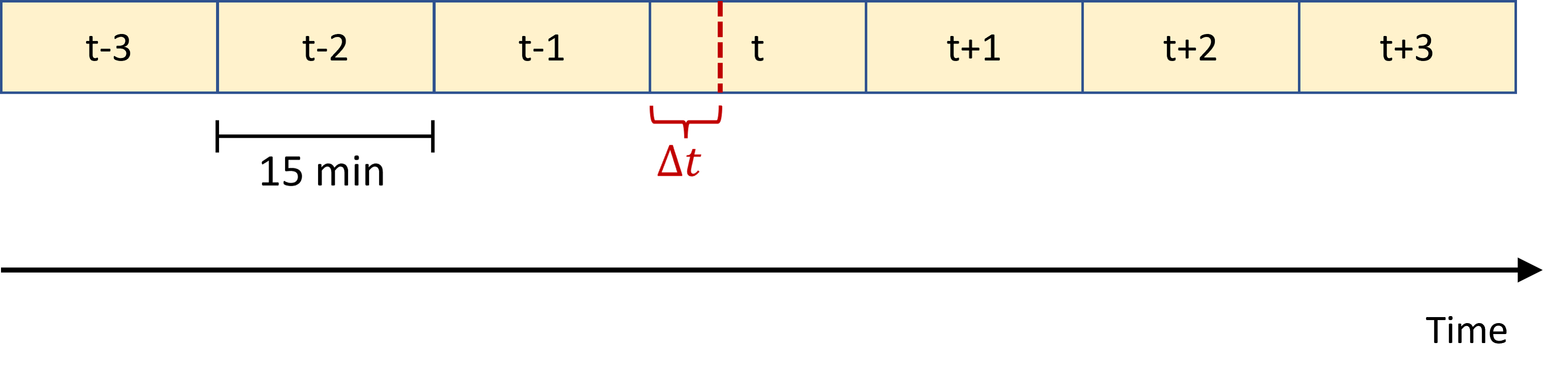
The Gridradar aFRR forecasting model aims to predict the direction of aFRR activation at time t, aFRR(t), which is a time interval Δt<15 min after the end of the last quarter hour, see the figure below. It is taken into account that the aFRR activation data of the different TSOs are published at different points in time. In order to always have the current status of the information available, the model therefore continuously checks which input variables are currently available.
In addition to data on aFRR activation, other frequency-dependent variables are included in the underlying model. Gridradar continuously records such frequency data with its own measuring stations distributed across Germany and Europe. The distributed measurement system enables comprehensive consideration of the current grid situation in Germany and in neighbouring countries. The combination of information from the TSOs and Gridradar's own measurements as well as other external input variables enables a precise forecast of the volume-weighted average of the direction of aFRR activation in the current quarter hour.
The aim of the forecast is to be able to provide additional information on the current and upcoming grid situation at short notice. The target group of the product are therefore mainly traders, balancing group managers and distribution system operators. The information provided by the aFRR forecast model enables interested parties to adapt their portfolio to the grid situation or to prepare or intervene at an early stage on the distribution grid side by means of appropriate switching.
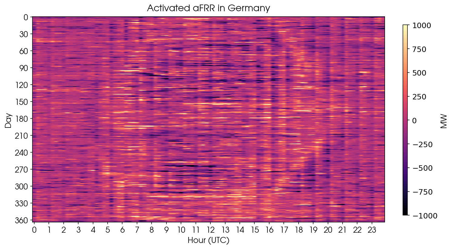
The figure below shows a diagram of the quarter-hourly averages of activated aFRR in Germany for the year 2021. The typical patterns known from grid frequency analysis (see here) are also observable in the aFRR activation. Two typical patterns stand out directly: hourly recurring patterns are due to trading artifacts, namely when power plants are ramped up or down at the hourly break or quarter-hourly break. Solar power production leads to aFRR activation at sunrise and sunset. This is shown by the "sun bulge" in vertical direction.
The total time period considered for the analysis of the model is January through October 2021. The figure below shows the distribution of the 15-minute average aFRR activations. In 53% of the cases, activation was negative, and in 47% it was positive. Overall, the distribution appears quite symmetrical.
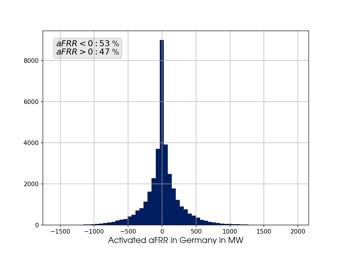
Accordingly, if a trader had expected continuous negative values for aFRR activation, she would have been correct in 53 percent of the quarter hours during the period under consideration. This means that the retrieval direction is approximately balanced. Thus, a trader would have optimized her portfolio approximately as well (or poorly) as if she had ignored the past aFRR data.
Combining the aFRR activation information with other current network information allows the forecast to be more precise. The degree of improvement and the robustness of the information will be demonstrated below.
To analyse the performance of the forecast, a model was trained with data from January to August 2021 (training set). Subsequently, the model was tested with aFRR data between September and October (test set).
Output and performance of the Gridradar forecasting model
Taking into account the availability of information and the resulting added value, the highest accuracy was achieved for Δt=10 min with a forecast accuracy of 81.5 percent. This does not change for a different choice of training and test sets - roughly the same accuracy was achieved for test sets from November to December and for January 2022, respectively, demonstrating the robustness of the model even in the face of changing environmental factors, such as those caused by holidays or seasonal weather conditions.
The Gridradar forecast model assigns a probability to the expected aFRR activation direction. The more predictable the forecast period, the higher the probability. A comparison of that probability and the realized aFRR activation shows that particularly high probabilities are associated with strong aFRR activations. Lower probabilities, on the other hand, indicate that the level of aFRR activation is less predictable. Estimating a probability has the advantage that decisions can also be made based on that probability.
The figure below on the left shows the predicted probability of a positive activation in the test set compared to the actual aFRR data. The horizontal axis represents the actually activated amounts, and the vertical axis the probability of a positive aFRR activation according to the model. The figure on the right shows the corresponding probabilities for negative activation.
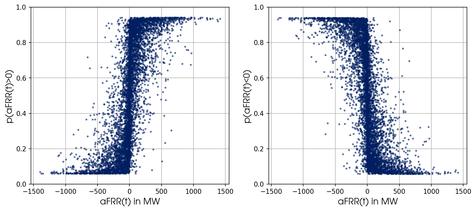
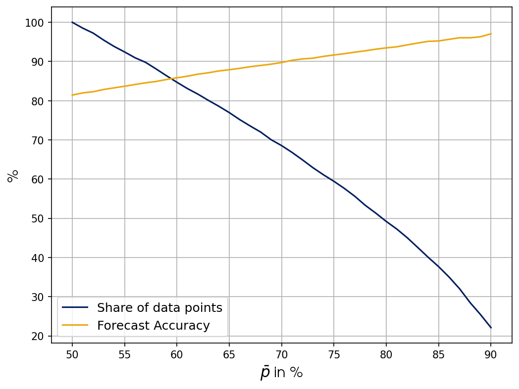
Looking first at the tails of the distribution, we see that high (positive and negative) aFRR values are easier to predict than low ones (close to 0). For example, if we restrict ourselves to the cases in the test set for which a retrieval direction is predicted with a probability of more than 65% (called p̅ in the following), which corresponds to 75% of all samples in the test set, this results in a correct prediction of the activation direction of more than 87%. This is illustrated below for different probabilities. For p̅=50% a positive or negative direction is predicted for every sample in the test set. Thus, the left end of the figure corresponds to the entire model. If we restrict ourselves to cases with a correspondingly higher prediction probability, we also obtain significantly higher accuracies.
Forecast accuracy and time of prediction
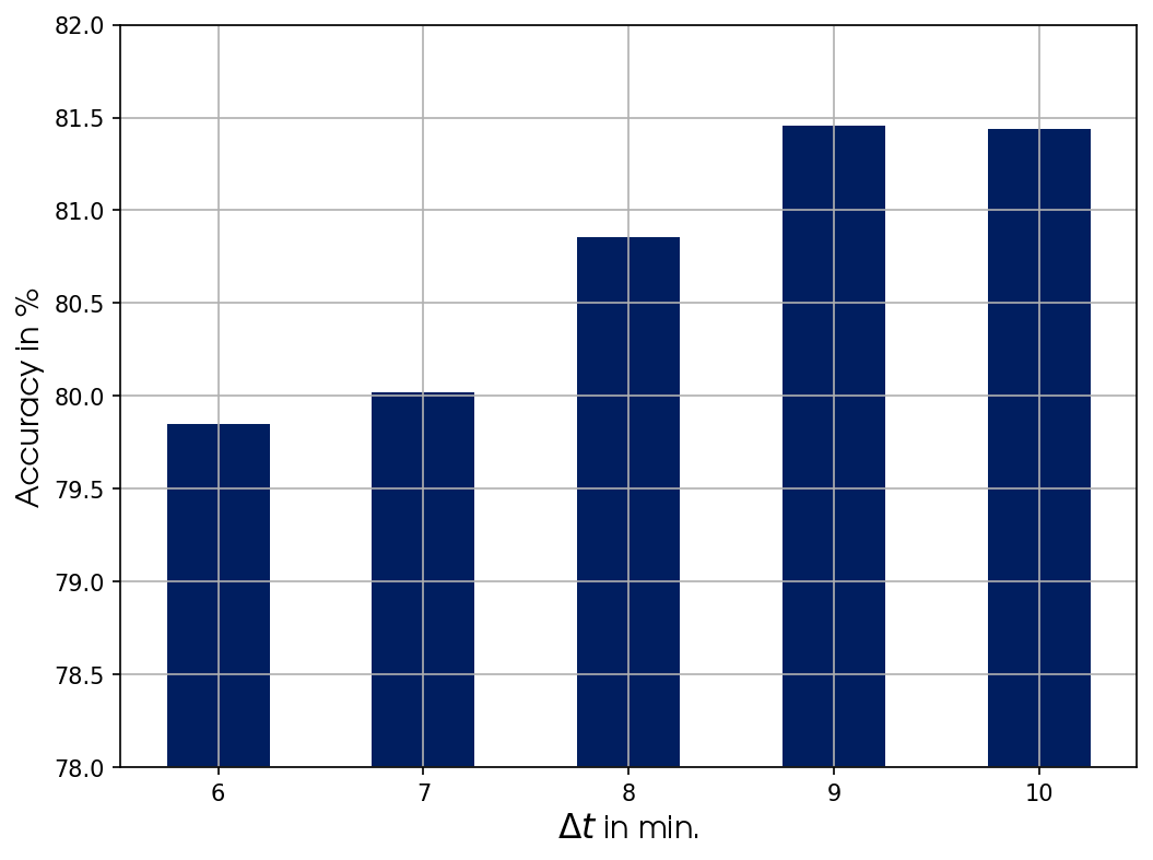
If we examine the performance of the forecast as a function of Δt, taking into account the operator-dependent publication times of the aFRR data, we see that our forecast is already 79.5% accurate for Δt=6 minutes. For Δt=10 minutes, the maximum accuracy is achieved with 81.5%. After that, there was no further improvement, which is probably due to the 5-minute full activation time for aFRR.
Summary and outlook
The preceding analysis shows that it is possible for traders, balancing group managers and power plant operators to adjust their portfolios to the grid situation at short notice. However, publicly available information from network operators is not sufficient for this purpose. Only the combination with further real-time information makes it possible to reoptimize the portfolio punctually on time before the end of the current quarter hour. This has two positive effects: On the one hand, it reduces costs for balancing group managers. This is because the allocated imbalancing energy costs can be massively reduced. On the other hand, the grid-serving optimization of the operating mode reduces the overall demand for balancing power. Passive balancing is not yet provided with financial incentives in Germany, as it is in the Netherlands, for example. Nevertheless, intelligent short-term management using real-time information about the grid offers potential savings for portfolio managers.